The weekly supply-demand balance's blind spot

Rising gas-fired generation is breaking backward-looking models

Throughout the shale era, US gas production has not only been the most important market driver but also the hardest to track in real time. For LNG and piped imports and US domestic consumption, pipeline scrapes and EIA daily generation data provide reliable real-time indicators of underlying fundamentals. But we don’t get a reliable read on dry gas production until the EIA-914 comes out three months later, so the weekly EIA gas storage number is the best quasi-real-time indicator of Lower-48 gas production.

But extracting a real-time read on production requires properly accounting for weather impacts, and that normalization is getting harder with rising gas-fired generation.

Building a supply-demand balance

Isolating underlying structural trends requires first accounting for cyclical factors — both direct weather impacts on demand and other seasonal factors, such as LNG maintenance or nuclear refueling outages. For the former, we build a linear model of gas storage injections as a function of heating-degree days, cooling-degree days, and holidays¹ over the 2021-25 period. The residual of this model is the gas supply-demand balance, an indicator of underlying market strength or weakness. Because each week’s observation is noisy, analysts typically smooth the time series with an exponential function.

Figure 1 | Gas supply-demand balance

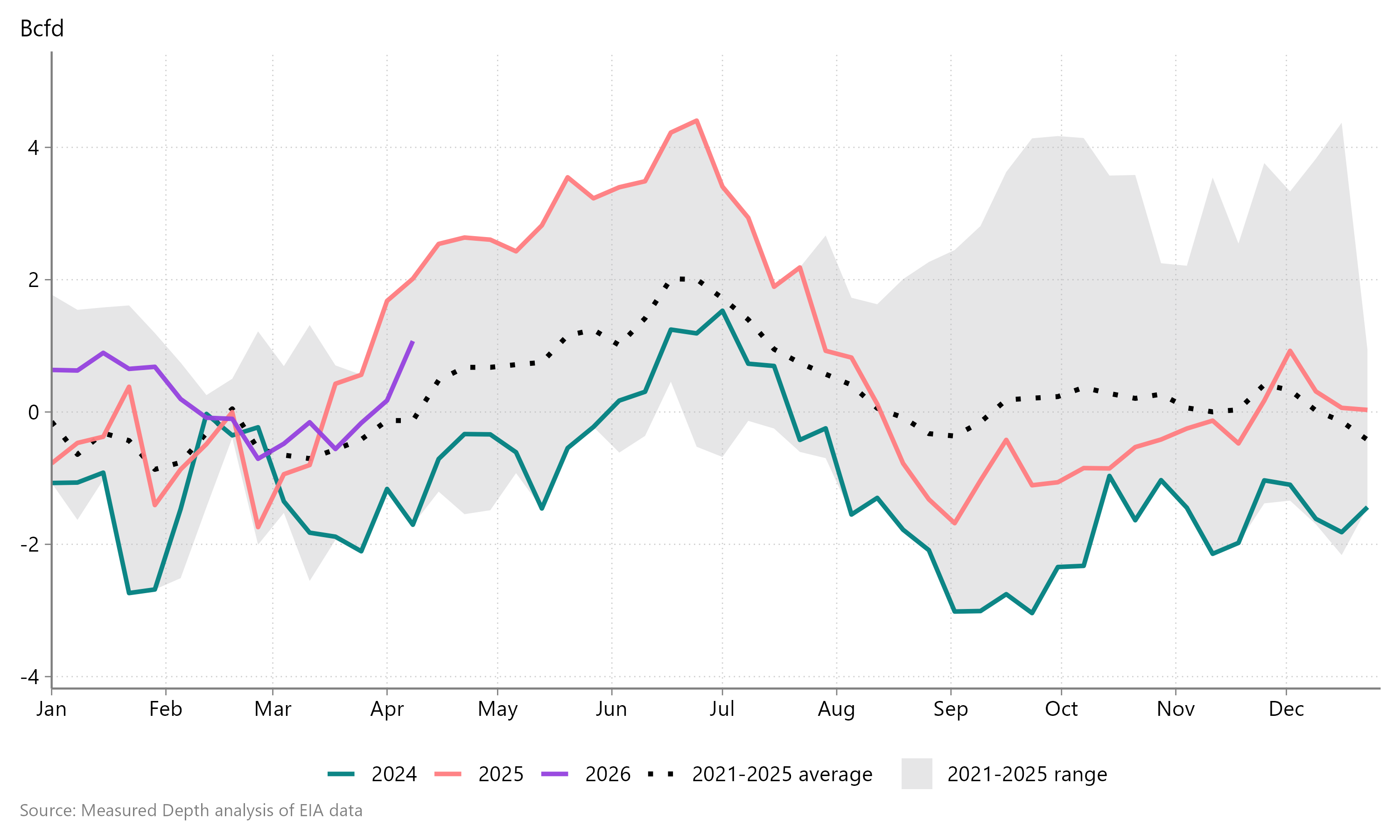
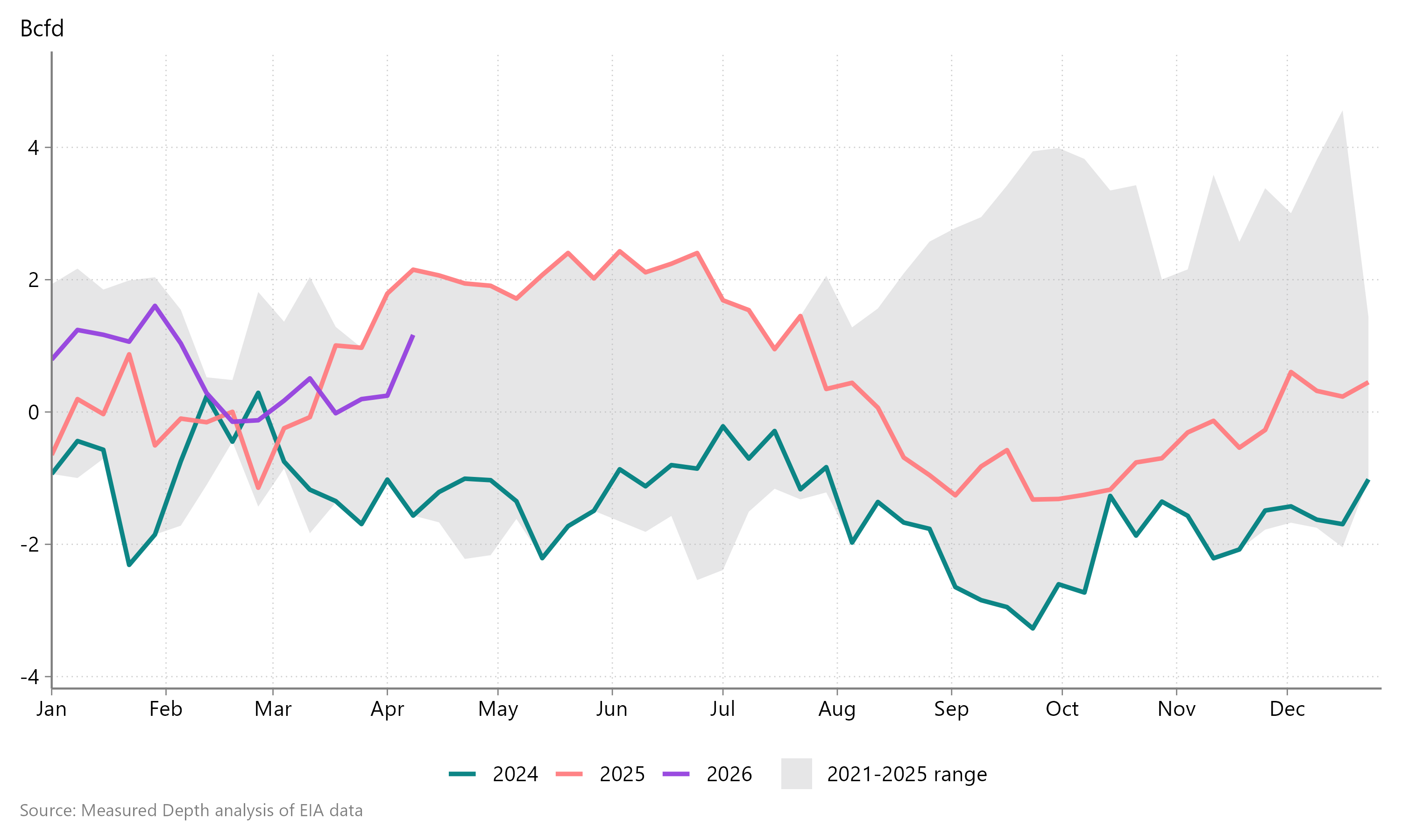
But the resulting indicator still varies throughout the year because non-temperature-related seasonal factors systematically tighten or loosen the gas market at specific times, such as nuclear refueling outages, wind capacity factors, and LNG maintenance. To correct for this seasonality, we net off the five-year² average supply-demand balance for that week to get a more neutral supply-demand balance.

Figure 2 | Seasonally adjusted gas supply-demand balance

How are changes in the gas market affecting the storage number?

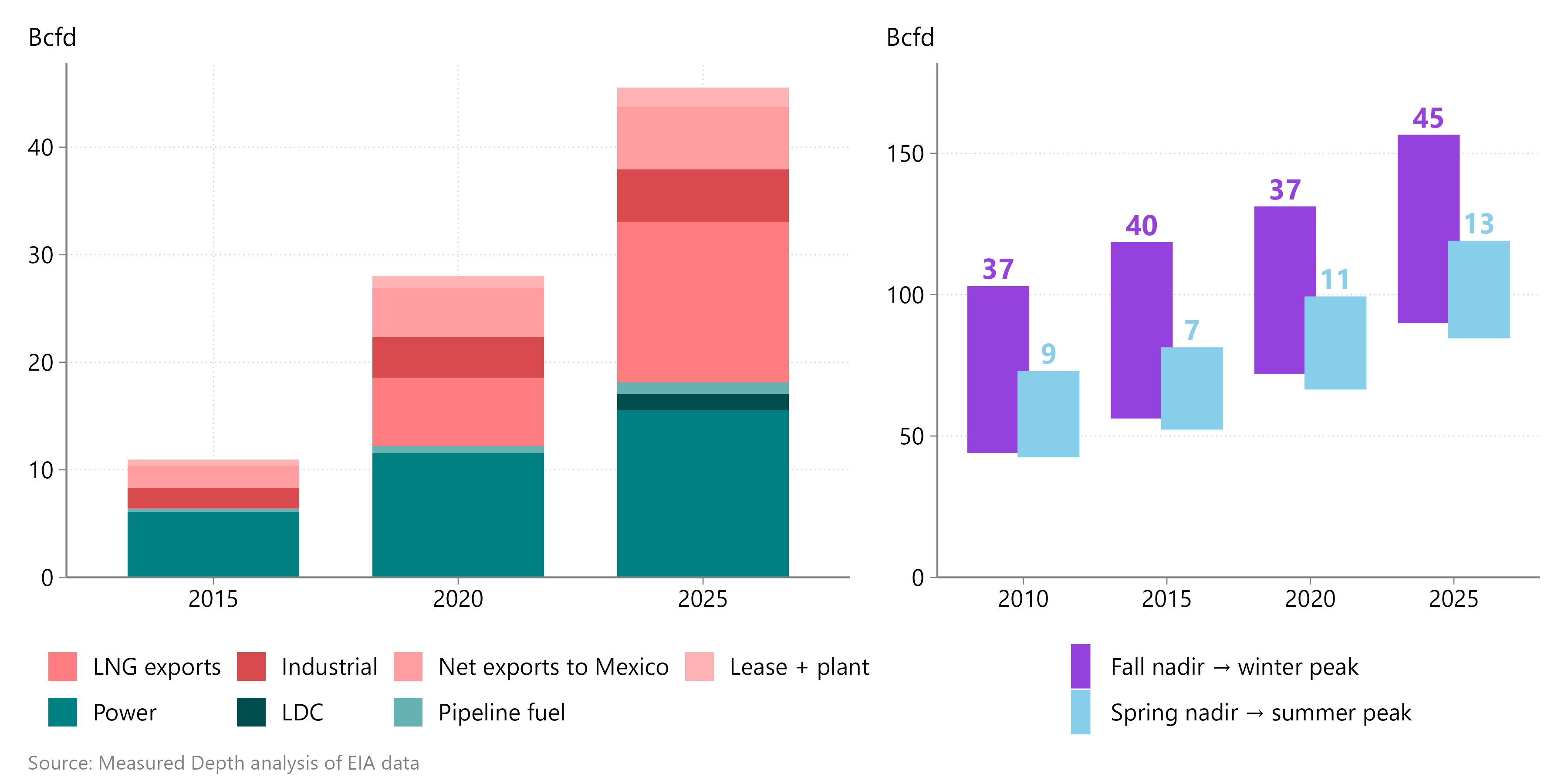
The rise in gas-fired generation means the absolute seasonality of US gas demand is nonetheless increasing, even as the plurality of US gas demand growth has come from LNG exports. Weather-sensitive gas demand — shown in the teal shades in Figure 3 — grew 18 Bcfd from 2010-25.

Figure 3 | US gas demand growth and seasonal range

This growth in weather-sensitive consumption — particularly power generation — means that the impact of degree days on gas burn will increase over time. And if instead of modeling the impact of weather on weekly storage injections over the 2021-25 period, we use shorter, rolling horizons, we can see how the relationship between weather and demand has changed over time.

Here, we face a tradeoff between using the most recent data and having enough data points to reliably estimate coefficients. A two-year sample probably does not have sufficient resolution for a reliable model, but even a three-year rolling horizon shows a consistent increase in the impact of cooling degree days, offset by a higher constant, meaning higher injections in a mild week.

Interestingly, HDD coefficients have stabilized in recent years, even as rising power generation has added demand that is sensitive to cold weather. I expect the HDD coefficient is not rising because gas pipeline capacity — contracted by LDCs — limits gas-fired generation on the coldest days.

Figure 4 | Rolling horizon coefficients

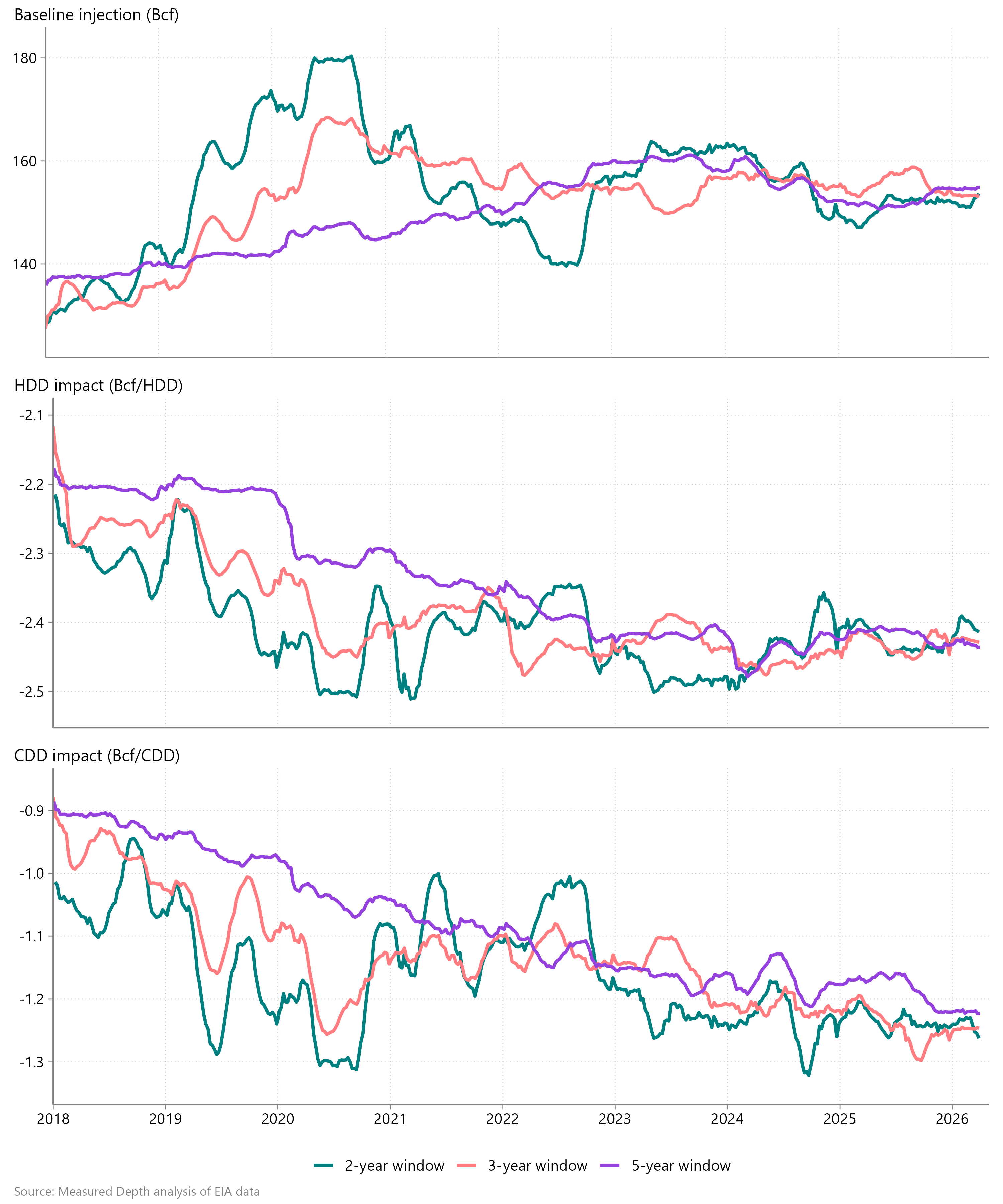
The self-correcting seasonal adjustment partially masks this drift, but not fully, because both the model and its seasonal adjustment are backward-looking — we should expect today’s true CDD coefficients to be higher still.

Forward-looking implications

The US gas market grew 70% over the last 15 years, while US underground storage capacity remained essentially unchanged. EQT and others have rightly pointed out that the same storage inventory levels provide much less of a cushion against gas market dislocations from weather, outages, or other factors. Rising gas-fired generation, meanwhile, means that the call on gas storage is nonetheless increasing. The result, then, is that modest dislocations between supply and demand can quickly lead to extreme price outcomes.

Now, a colder-than-normal winter draws down storage inventories much more quickly; similarly, producers’ outrunning demand by a small percentage risks quickly creating a storage glut. So while the EIA’s gas storage number, released each Thursday morning at 9:30 CT, has always been the biggest needle-mover for NYMEX Henry Hub prices, it is now more important than it has been at any time since the pre-shale era, when supply and demand elasticity were much weaker.

The rise in weather-sensitive demand means that models built on lagging data — which is all of them! — will, in summer months, under-predict the impact of each CDD and therefore under-attribute demand to the weather and over-attribute it to structural strength (and conversely in the spring and fall). In other words, a hot July week looks structurally tighter than it really is, and a windy April one looser.

And while we’re mostly looking at the supply-demand balance for a read on production, understanding the level of gas-fired generation in a given week is different than isolating what that means for the future. In the next installment of this series, I’ll show how the rise in renewable generation overstates market looseness in the spring and tightness in the summer.

1. To identify which holidays are significant, I analyze daily pipeline scrape data

2. I’ve also seen firms use other time horizons, but the principle remains the same